Introduction
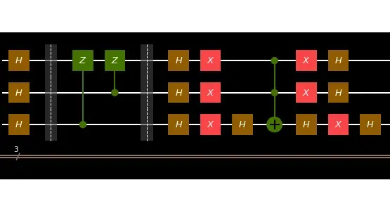
This article goes through the Qiskit Textbook Grover’s algorithm explaining it in more details, showing how to apply quantum Gates as the matrix calculus. Before going further with this tutorial, you should get familiar with the theoretical Introduction in the Qiskit Textbook. Grover algorithm is being described as a searching algorithm for the unstructured database. However, this example shows, how to perform the Groover’s algorithm, to make a quantum system to reveal the marked states.
Preparation part
(For the first time I suggest to skip directly to the Example)
Quantum Gates as matrices
import numpy as np
from qiskit.extensions import HGate, CnotGate, IdGate, XGate, CzGate, ZGate

# |0>, |1>
zero = np.array([[1.],
                 [0.]])

one = np.array([[0.],
                [1.]])

# Gates: I, Z, H, X
I = IdGate().to_matrix()
Z = ZGate().to_matrix()
H = 1./np.sqrt(2) * np.array([[1, 1],
                              [1, -1]])
X = XGate().to_matrix()

# 3-qubit Hadamard gate
Hq012 = np.kron(np.kron(H,H),H)

# 3-qubit CZ gates
p00 = zero * np.array([1, 0]) # |0><0|
p11 = one * np.array([0, 1]) # |1><1|
# control = 1 (|0><0| + |1><1|), target = 0 (Z), uninvoled =2 (I)
# 012 + 012 - qubit indexint
cz10 = np.kron(np.kron(I, p00), I) + np.kron(np.kron(Z, p11), I)
cz20 = np.kron(np.kron(I, I), p00) + np.kron(np.kron(Z, I), p11)

# 3-qubit CCZ gate
# control = (|0><0| + |1><1|),
# target = (Z)
# control = 21
# target  = 0
ccz210 = np.kron(np.kron(I, p00), p00) + np.kron(np.kron(Z, p11), p11)
qiskit:
# initialization
import matplotlib.pyplot as plt
%matplotlib inline

# importing Qiskit
from qiskit import IBMQ, BasicAer
from qiskit import QuantumCircuit, ClassicalRegister, QuantumRegister, execute

# import basic plot tools
from qiskit.tools.visualization import plot_histogram
Example
According to the example we have got a three-qubit qubit system and we want to make it return our two marked states: and .
The whole procedure is as follows:
- Prepare the quantum system
- Create superposition of states
- Run the oracle over the system
- Amplify the amplitude
1. Prepare the quantum system
Combine 3 qubits in state |0> to make one qbyte register:
matrix:
state = np.kron(np.kron(zero, zero), zero)
state
array([[1.],
[0.],
[0.],
[0.],
[0.],
[0.],
[0.],
[0.]])Note that you can treat it is as a bit string, calculating the value of the state form binary to decimal
(eg. ), the result is pointing you the position of the 1 in the vector (on the 0th or 5th position accordingly).
qiskit:
q = QuantumRegister(3)
c = ClassicalRegister(3)
circ = QuantumCircuit(q, c)

circ.draw(output='mpl')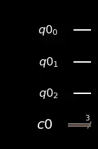
2. Superposition
Apply Hadamard gates to the qubits to create a uniform superposition:
matrix:
state = np.dot(Hq012, state)
state
array([[0.35355339],
[0.35355339],
[0.35355339],
[0.35355339],
[0.35355339],
[0.35355339],
[0.35355339],
[0.35355339]])
qiskit:
circ.h(q)
circ.draw(output='mpl')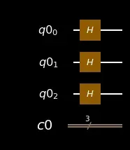
** 3. Oracle **
Mark the desired states and using a phase oracle:
you can see, that the marked states where flipped.
matrix:
oracle =cz20*cz10
state = np.dot(oracle, state)
state
array([[ 0.35355339+0.j],
[ 0.35355339+0.j],
[ 0.35355339+0.j],
[ 0.35355339+0.j],
[ 0.35355339+0.j],
[-0.35355339+0.j],
[-0.35355339+0.j],
[ 0.35355339+0.j]])
qiskit:
circ.barrier() # for readabilty
circ.cz(q[2], q[0])
circ.cz(q[1], q[0])
circ.draw(output='mpl')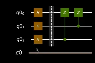
4. Amplify probabilities
4a). Apply Hadamard gates to the qubits:
matrix:
state = np.dot(Hq012, state)
state
array([[ 5.00000000e-01+0.j],
[ 0.00000000e+00+0.j],
[ 2.77555756e-17+0.j],
[ 5.00000000e-01+0.j],
[ 5.00000000e-01+0.j],
[ 0.00000000e+00+0.j],
[ 2.77555756e-17+0.j],
[-5.00000000e-01+0.j]])
qiskit:
circ.barrier() # for readabilty
circ.h(q)
circ.draw(output='mpl')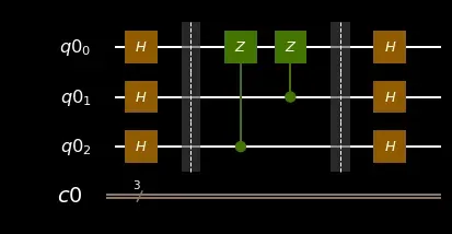
4b). Apply X gates to the qubits:
Xq012 = np.kron(np.kron(X,X), X)
state = np.dot(Xq012, state)
state
array([[-5.00000000e-01+0.j],
[ 2.77555756e-17+0.j],
[ 0.00000000e+00+0.j],
[ 5.00000000e-01+0.j],
[ 5.00000000e-01+0.j],
[ 2.77555756e-17+0.j],
[ 0.00000000e+00+0.j],
[ 5.00000000e-01+0.j]])
qiskit:
circ.x(q)
circ.draw(output='mpl')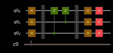
4c). Apply a doubly controlled Z gate between the 0, 1 (controls) and 2 (target) qubits
matrix:
state = np.dot(ccz210, state)
state
array([[-0.5+0.j],
[ 0. +0.j],
[ 0. +0.j],
[ 0.5+0.j],
[ 0.5+0.j],
[ 0. +0.j],
[ 0. +0.j],
[-0.5+0.j]])
qiskit:
# There is no ccz gate in qiskit so we need to implement it using h-ccx-h
circ.h(q[2])
circ.ccx(q[0], q[1], q[2])
circ.h(q[2])
circ.draw(output='mpl')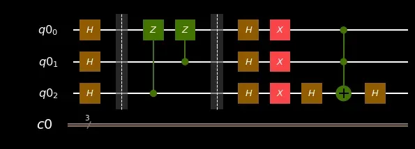
4d). Apply X gates to the qubits
matrix:
state = np.dot(Xq012, state)
state
array([[-0.5+0.j],
[ 0. +0.j],
[ 0. +0.j],
[ 0.5+0.j],
[ 0.5+0.j],
[ 0. +0.j],
[ 0. +0.j],
[-0.5+0.j]])
qiskit:
circ.x(q)
circ.draw(output='mpl')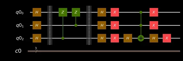
e). Apply Hadamard gates to the qubits
matrix:
state = np.dot(Hq012, state)
state
array([[ 0.00000000e+00+0.j],
[ 9.52420783e-18+0.j],
[ 9.52420783e-18+0.j],
[ 0.00000000e+00+0.j],
[ 0.00000000e+00+0.j],
[-7.07106781e-01+0.j],
[-7.07106781e-01+0.j],
[ 0.00000000e+00+0.j]])Results 5: |101>, 6: |110>.
(look carefully that states 1 = |001>, and 2 = |010>, are almost equal to 0).
qiskit:
circ.h(q)
circ.draw(output='mpl')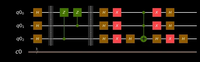
circ.measure(q, c)
backend = BasicAer.get_backend('qasm_simulator')
shots = 1024
results = execute(circ, backend=backend, shots=shots).result()
answer = results.get_counts()
plot_histogram(answer)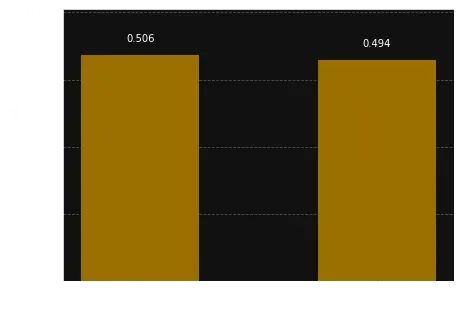
Conclusion
The example above shows how to apply Grover’s procedure over the quantum system. The system returns the states that we already know. More oracles for the qubit system you can find in “Complete 3-Qubit Grover search on a programmable quantum computer”, eg.:
The real advantage of this algorithm is when we know only some constraints for the results, and we can design appropriate oracle so the algorithm can give us as output the solution. For example, for the database search, we describe only some attributes of the elements, and the system returns us the addresses of the elements that should be retrieved.
Go to the current Jupyter Notebook to evalute code in this text.
Refferences
- Qiskit Textbook Grover’s algorithm
- C. Figgatt, D. Maslov, K. A. Landsman, N. M. Linke, S. Debnath & C. Monroe (2017), “Complete 3-Qubit Grover search on a programmable quantum computer”, Nature Communications, Vol 8, Art 1918, doi:10.1038/s41467-017-01904-7, arXiv:1703.10535
- Łukasz Herok, Compressing bit strings in qubits using superposition effect