On a Friday afternoon, Mr Zenon, production manager at the fictional company MetalTech, receives an urgent order. Three parts, three machines: a lathe, a milling machine, a welder. Every part goes through the machines in the same order, and each operation has a different processing time. The question is simple: in what order should the operations be placed on the machines so that the whole order is finished as soon as possible?
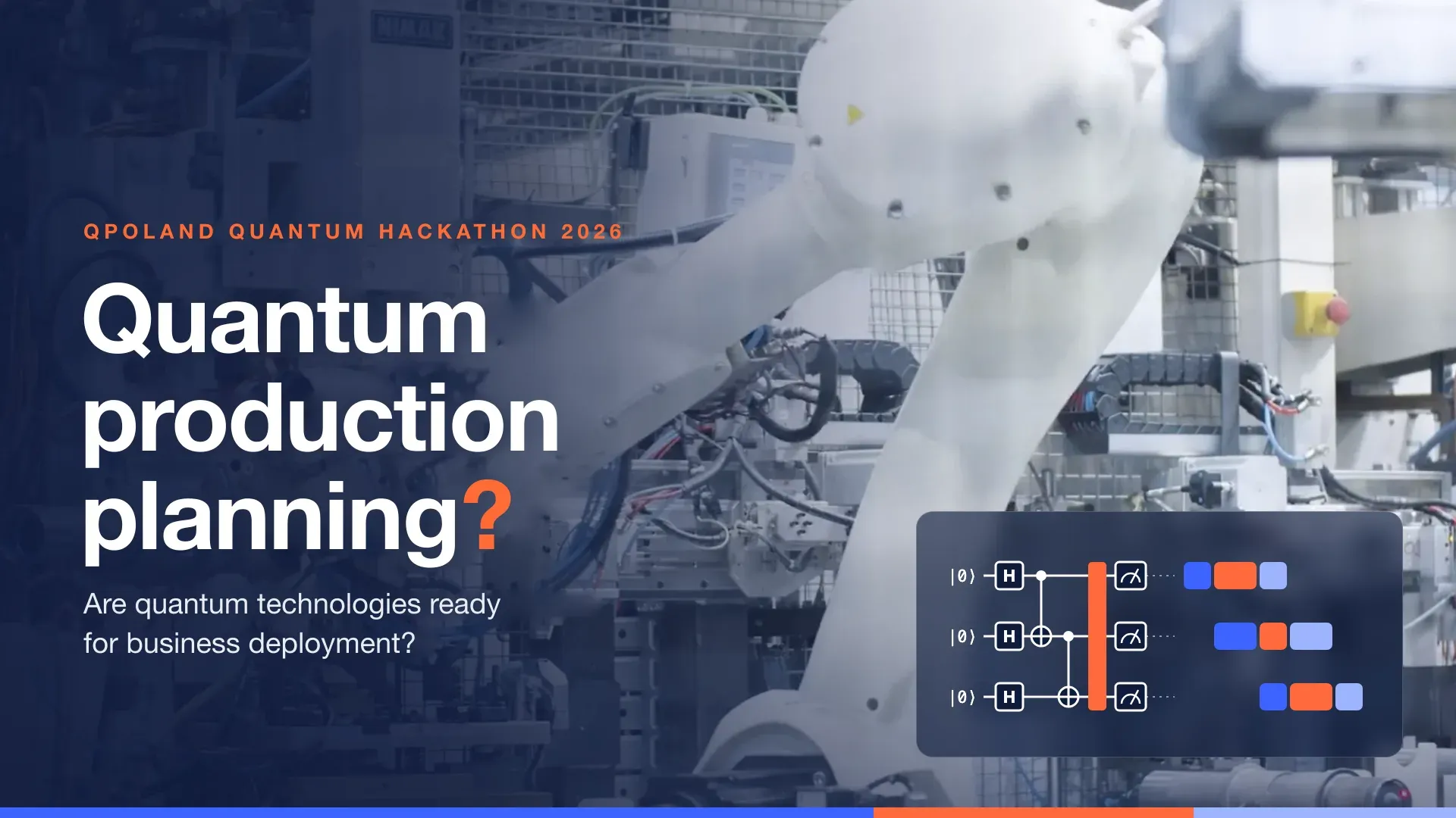
A few days later Mr Zenon had nine plans from the teams of QPoland Quantum Hackathon 2026. All of them optimal.
My day job is designing an ERP system, so production planning is, for me, one algorithm among many. I prepared this task for the hackathon, which my company KLL-ERP supported, with a single question in mind: do quantum methods give us anything more here today than an ordinary computer?
The short answer to the question in the title is: no, not yet. But the road that shows it is far more interesting than the bare “no”.
Nine teams submitted projects [1]. I ran every codebase in an isolated environment and recomputed the key numbers independently. Where that was not possible, I say so explicitly. Numbers in square brackets refer to the list of sources at the end.
If you come across an unfamiliar term, such as QUBO, QAOA or qubit, click it in the text or see the glossary at the end of the article.
The task was deliberately small
The hackathon had two stages [14]. The first, mandatory one was an entry ticket: two small instances of the problem.
- Instance A: 2 jobs on 2 machines, the optimal plan takes 4 hours. Written as a QUBO, after discarding impossible start times, it has about 8–12 binary variables. In a direct encoding each variable is one qubit, so such a circuit can be simulated on a laptop. Here the teams had to solve the QUBO with a quantum algorithm, usually QAOA, on a simulator or on real hardware.
- Instance B: 3 jobs on 3 machines, the optimal plan takes 8 hours. In the time-indexed formulation, where each variable says whether a given operation starts at a given hour [15], the QUBO has 72 variables, and 39 after discarding impossible start times [14]. A full simulation of 39 qubits would need about 8 TiB of memory. That is already too much for an ordinary computer.
QUBO is the format accepted by a quantum annealer and by QAOA [2, 6], so the teams built their models in a language a quantum computer can understand. Moving such a model onto real hardware is not free, though. It has to be fitted to the connections between qubits, which usually adds qubits or gates [16, 17].
Today we solve such models classically, for example with VeloxQ. The reason is not the number of qubits as such, since today’s processors have more than a hundred [18]. Noise matters more. Today’s quantum processor is like a machine with a high scrap rate: the longer the operation, the more likely the part comes out defective. Theoretical analyses show that under typical noise models, deep optimisation circuits give no clear advantage over classical methods until error rates drop by orders of magnitude [11]. That is why the teams fought for what counts on any quantum computer: the smallest model that is still exact. In a direct encoding, every variable saved is one qubit fewer.
The second stage was the main part of the competition. Each team extended the problem in its own way: adding due dates, changeovers, machine breakdowns, more jobs, or looking for ways to fit the problem onto fewer qubits.
Everyone was right. And that was the first warning sign
All nine projects reached the optimal plans: 4 and 8 hours. At first glance, a success. At second glance, a question appears: if everyone was right, what actually distinguishes the methods?
The answer is uncomfortable for me as the author of the task. The 3x3 instance turned out to be both too easy to prove anything and too large to compute directly on a quantum computer.
In this type of problem (a so-called flow shop) it was enough to choose the order of jobs, shared by all machines [19]. For two machines a simple rule by Johnson gives it [20], and from three machines on the problem is NP-hard in general [21]. So it was our instance that was easy, not the problem as a whole.
Three jobs can be ordered in only 6 ways, and as many as 4 of them give the optimal 8 hours. It is like a multiple-choice test where four of six answers are correct. A randomly chosen order hits the optimum 67% of the time. On the 2x2 instance there are two orders, so a coin toss gives 50%.
The same task written as start times looks different. Among 512,000 assignments in which every operation starts exactly once (after pruning impossible hours), only 13 are valid plans. Here random guessing practically never hits.
Except that this formulation needs 39 qubits, too many for a straightforward simulation and for today’s noisy hardware [17, 11]. So the teams faced a choice: an encoding on a few qubits, where even random guessing finds the optimum, or the full encoding, which can neither be simulated directly nor run reliably on today’s hardware. Only one project fitted between these extremes with a clear effect. I will come back to it shortly.
In a small encoding, an algorithm that does nothing meaningful still often “finds” the best plan. The chance that independent attempts contain at least one success is . When drawing orders at random (), 6 attempts are enough for about a 99.9% chance of the optimum. So “it found the optimum” proves nothing on its own. In two projects the code mapped any bit string to some valid order and then computed its makespan. With such a decoder, a random bit string hit the optimum 75–81% of the time. In one of those projects, more often than the quantum algorithm’s own output.
So for the following projects I stopped asking whether the result was good. I asked: who actually computed this plan, the quantum algorithm or the ordinary computer next to it?
Where the quantum computer really does the work
This was the most interesting part of the evaluation. Several patterns kept recurring in which the result formally came from a “quantum method”, but classical code did the decisive work. Not all of them are mistakes. Some are normal, sound elements of a hybrid approach. You just have to see them before giving the quantum computer the credit.
The answer baked into the formula. Imagine a planner who first computes, in Excel, the duration of every possible order, and then asks a new system to pick the best one from that table. The system “found” the optimum, but Excel did the work. The smallest encodings represented the 2x2 problem on 1 qubit and 3x3 on 3–4 qubits. Impressive, until you look at where the coefficients come from. In several projects the code first computed the makespan of every order and then built the energy function from that table. Computing coefficients classically is normal in itself. The problem is the exhaustive enumeration: whoever has computed the makespan of every order already knows the best one. For 3 jobs that is 6 evaluations; for 20 jobs it would be about 2.4·10¹⁸, before the quantum computer even starts. Some teams, including the winners, openly described such an encoding as a comparison point rather than the actual model.
The best sample out of almost all possible ones. Roll a die a hundred times and a six will almost certainly come up. That does not mean you know how to roll. QAOA does not return a single result but a distribution of measurements: thousands of bit strings, some appearing more often, others less. Picking the best of many samples is a standard part of optimisation, because checking a single plan is cheap [6]. The trouble starts when there are so many samples that they cover almost the entire space of possibilities. In the extreme case the code went through all 16 possible states of a 4-qubit circuit, which is just an ordinary classical search. A fair comparison is the best result of the quantum algorithm from samples against the best of random samples, and, in a practical evaluation, the total computation time as well [22].
A hint that is already the answer. Give a new planner a ready-made best plan and ask them to improve it. They will return the same plan and, formally, be right. Warm-starting, i.e. starting the quantum algorithm from a solution suggested classically, is a legitimate technique [23], but what counts is how much the algorithm improved. In two projects the starting point was already the answer. In one, the initial state alone gave about 91% optimal measurements, and 99% after optimisation: the plan was found by the classical stage before the quantum algorithm.
A horizon equal to the known optimum. Tell a planner “fit everything into 8 hours” when you already know that 8 hours is the best possible result. Every plan that fits will be optimal. The time-indexed QUBO model used here needs an assumed horizon [15]. Searching for the smallest feasible , starting from a lower bound, is a correct optimisation method, and that is what the best teams did. It is different when is set exactly to the optimum computed beforehand by a classical solver. Then a table showing “0% gap to optimum” follows from the construction, not from the quality of the solver.
Classical preprocessing. A good process engineer first crosses out the variants that cannot be produced and only then hands the task to the planner. That is good practice, but the credit goes to the engineer, not the planner. The best projects shrank the problem substantially by classical means before it reached the quantum algorithm. In one team, pruning start windows and constraint propagation [24, 25] reduced the number of assignments in which each operation starts exactly once from 134 million to about 104 thousand, roughly 1,300 times. The quantum algorithm then searched for 13 valid plans among those 104 thousand. The same reduction also helped classical methods: simulated annealing hit the optimum in 40% of runs on the full model and in 97% on the reduced one. A fair benchmark gives classical methods the same preprocessing.
What is left once these effects are separated?
It is clearest as a funnel.
| Question | Projects |
|---|---|
| Reached the optimal plans of 4 h and 8 h | 9 of 9 |
| Solved the 3x3 instance with a quantum algorithm on a classical simulator (the rest: classical annealing or a MILP solver, plus VeloxQ) | 5 of 9 |
| … of which QAOA without coefficients computed by enumerating all orders | 2 of 9 |
| … of which with a total probability of an optimal plan clearly higher than random guessing | 1 of 9 (about 1,400 times) |
| On the smaller 2x2 instance: QAOA on the full time-indexed model (8–12 qubits) that produced the reported result by itself, without hints from enumerating all states, clearly better than random guessing | 4 of 9 (about 8–400 times) |
“Probability of an optimal plan” is the total probability of all optimal plans in a single sample.
That one project out of nine is stegoqubit. The team reduced the 3x3 QUBO from 72 to 33 variables without losing a single valid plan, and ran on it a variant of QAOA with an XY mixer [26, 27]. The algorithm starts from states in which each operation starts exactly once, and the XY mixer does not break that rule. The total probability of the 13 optimal plans was 17.2%, about 1,400 times more than picking one of the 104 thousand assignments at random. The nine most frequently measured states were all optimal schedules. Separately, the team went down to as few as 24 variables thanks to “domain-wall” encoding [28], but checked that version only classically. The QAOA result refers to the 33-variable model.
It is still worth asking: is there actually a quantum circuit here? For 3x3 the team computed the algorithm’s behaviour with numerical code, without noise, over all 104 thousand states. That is a correct way to study an algorithm, but it is not running it on a quantum computer. And the ratios, about 1,300 times from pruning and about 1,400 times from QAOA, are increases in the chance of hitting the optimum, not a computational speedup.
On the smaller 2x2 instance, a clear QAOA effect was also shown by the teams RafeyC and ls-QPoland (probability of the optimum 13–18 times higher than random, with the optimal plan as the most frequent measurement) and AI-Native Quantum (about 8 times, although the optimal plan was only the third most frequent result). These are not big numbers, but they are a genuine effect of the algorithm, not of the classical code around it.
Real hardware: what the IBM processors showed
Only one team, Prometheus, ran the problem on real quantum computers: three IBM Heron processors, about 147 thousand shots of a 4-qubit circuit. The team provided job IDs and screenshots from the IBM platform, and the raw results are statistically consistent with the circuit for the MetalTech task. I could not check the jobs on the IBM platform themselves, so I have proof that the data is consistent, but not of where it came from.
The distribution of results from the hardware was very close to the ideal one. The similarity measure reported by the team (the squared Bhattacharyya coefficient) was 0.90–0.97, where 1 means identical distributions. Completely random results would give about 0.56. The hardware faithfully executed the technical drawing.
The trouble is that the drawing itself added little. The team’s decoder mapped every 4-bit string, including invalid ones, to some job order. With that decoder, the optimal plan came out in about 60% of the ideal circuit’s measurements, in 55–66% on hardware, and in 81% of random bit strings (13 of 16). Counting only strings that are themselves a valid and optimal order, the circuit did beat random guessing: 57% in the ideal simulation and 47–51% on hardware, against 25%. Across the team’s whole pipeline, however, the quantum part did not improve the result.
The conclusion cuts both ways. On a few qubits, today’s hardware gave results close to the simulation and was accessible to a hackathon team over a single weekend. Cloud access itself is not new: IBM made a five-qubit processor publicly available as early as 2016 [29]. Since then, what has grown is mainly the number and quality of qubits and the maturity of the tools [18]. At the same time, 4 qubits is a problem a person can solve on paper. QAOA experiments on superconducting processors show that result quality falls as the problem grows, especially when its structure does not match the connections between qubits [17].
VeloxQ: inspired by physics, computed classically
The most practical results came from a tool that is not a quantum computer at all. VeloxQ is a Polish QUBO solver from Quantumz.io, based on physics-inspired heuristics and running on ordinary CPUs and GPUs [12, 13]. It accepts the same problem format as a quantum annealer, but handles problems far larger than today’s quantum computers.
What the projects showed:
- On the official 3x3 instance (24–72 variables, depending on the encoding), VeloxQ, according to the recorded results, found the optimal plan on every call.
- The AI-Native Quantum team ran two campaigns on models of up to 128 variables. VeloxQ hit the optimum confirmed by CP-SAT in 3 of 4 cases in the first and in all 4 in the second. The share of feasible samples, however, fell from about 90% to about 20% as the problem grew.
- With hundreds and thousands of variables, the trouble began. In one project, VeloxQ run on the whole model was, from 8 jobs upwards, 22–59% worse than the optimum that CP-SAT proved in under 2 seconds. In another, VeloxQ alone returned mostly empty plans.
- It started to compete with classical methods only together with a classical loop that splits the problem into smaller pieces and stitches the results together (large neighbourhood search, LNS [30], or decomposition). In the project of the winners, team Axion, which modelled a catering kitchen instead of a factory, the VeloxQ + LNS hybrid on models of up to about 2,000 variables was one batch of meals better than the classical CP-SAT solver [31] with a 30-second limit, but worse than the same CP-SAT with a 4-minute limit. This is a comparison with time-limited results, not with a proven optimum.
For me this is the most instructive part of the hackathon. Both teams that received the VeloxQ award, Axion and stegoqubit [1], showed not only where the solver helps but also where it loses.
The price of realism, or why a real factory does not fit into qubits
The rules asked teams to count how many variables each new constraint costs. From an ERP perspective this is one of the most valuable lessons of the hackathon, because it shows what happens to the model when we add the real life of a factory to it.
In the time-indexed formulation used by most teams, the number of variables grows as the number of operations times the number of possible start times [15]. For 3 jobs on 3 machines that is 72 variables, 39 after pruning impossible hours [14]. Every extension of the horizon, every additional machine and every job increases that number. And because more jobs also need a longer horizon, it grows faster than the number of jobs itself.
Examples from the projects:
- Team Axion’s catering-kitchen model would need 1,118 variables in the time-indexed formulation. A clever reformulation brought it down to 35.
- Stegoqubit’s extended factory model with changeovers, machine maintenance and due dates went from 102 to 24 variables thanks to classical constraint propagation and “domain-wall” encoding, without losing a single valid plan.
- Tardiness penalties and time-of-use energy costs, computed from the existing start variables, did not cost a single extra variable. Not every business requirement is expensive. A hard deadline would be different: a constraint that removes some of the possible start times.
- Machine breakdowns reduced the number of variables, because they removed impossible start times, but they lengthened the required horizon. On balance, the variable count could go up.
Then there are the penalties for breaking the rules. They work like a fine: they must be higher than the gain from breaking the rule, otherwise the solver decides it pays to break a factory rule. On the other hand, a penalty that is too high drowns out the differences between good and bad plans [3, 32]. In one project the penalty was about 11 million against an objective in the tens, which required separate work on the conditioning of the problem. So the fine can be neither too low nor so high that everything else gets lost in rounding.
The classical referee
One fact sums up the state of the technology well. In all nine projects, the optimality of the result was confirmed by a classical solver (CP-SAT from Google OR-Tools [31] or MILP) or by exhaustively checking all possibilities. Such a comparison is standard in a fair benchmark, but something else is telling. The same CP-SAT solves the 3x3 instance and the extended factory model with the status OPTIMAL, i.e. with a proof of optimality [33], in a fraction of a second. Random portfolios with 12 jobs, changeovers and due dates take it about 1.2 seconds (within the assumed horizon). Constraint programming solvers also cope with industrial-scale scheduling [34], although on large instances within a time limit they do not always prove optimality.
The best teams played with their cards on the table: they compared every quantum result with a classical one and reported the difference. According to a review of the field, such comparison with the best classical methods is one of the key open tasks of quantum optimisation as a whole [35]. The Neural Husars team went furthest in the other direction: they solved their QUBO with an exact classical solver and formally proved that it was the same problem. Announcements about “quantum optimisation” could use more of this practice.
AI wrote much of the code. That changes what needs checking
The rules allowed AI, and nearly all projects clearly used it. Copilot, Codex, Claude Code, Gemini and ChatGPT were named explicitly in the descriptions, and the repositories contained instructions for agents. In several projects the documentation states plainly that much of the code was written or generated by an AI agent. According to its team’s log, one complete and correct project was built in an hour and a half. Another amounted to almost 150 commits in three days and about 170 documents.
This shows two things. First, writing working quantum optimisation code is no longer a barrier. A baseline that a few years ago would have needed weeks of learning Qiskit is now built in an hour. Second, the risk grows that the documentation says something different from the code:
- In one project, the key numbers in the work log (almost 100% success) did not follow from the code, which gave about 30%.
- In another, a claimed 5.43% saving in energy cost turned out to be an artefact: the compared plans had the same score, and the code picked one of them arbitrarily. On a rerun the difference was zero.
- In yet another, the work log and the description of AI’s role were rewritten just before the deadline, and the new version contained wrong numbers.
I used AI myself during the evaluation (Claude Code), so AI was helping me check code written with the help of AI. That is why I ran every codebase in an isolated environment and recomputed the key numbers independently.
The lesson for anyone evaluating projects, offers or presentations in this field: generating a convincing quantum project is cheap today. Verifying it is expensive and rare.
The projects that scored highest on documentation were those that stated plainly what was quantum and what was classical, and whose numbers reproduced to the digit with the same random seeds. My observation from this evaluation: the projects that openly described their limitations were also the easiest to verify.
Is it ready for business?
Based on these projects, the answer comes in three parts.
For day-to-day production planning: no. None of the evaluated projects demonstrated a practical advantage of the quantum part over appropriate classical methods. A clear effect of quantum algorithms was visible only on problems with a handful of jobs, and only in simulation. Similar scales appear in the literature: for example, Kurowski and co-authors studied QAOA for job scheduling on a basic instance, in noiseless simulation [36]. In the time-indexed formulation a real production plan means thousands of variables. Smaller encodings and decomposition can reduce that, but no project showed that anything can then be gained over classical methods.
For hybrid work and analysis: partly yes, but not thanks to quantumness.
- Physics-inspired solvers such as VeloxQ run on ordinary hardware today. Combined with classical decomposition, they could compete with classical methods under a short time limit. It is a real tool for experiments, though not yet a replacement for CP-SAT.
- The most interesting business insights from the projects were classical, but came from a good model. Team Axion showed that a third stove does not increase the number of meals served, while an extra helper adds 20 more. Team AI-Native Quantum showed that the shortest plan is not always the best when tardiness and energy costs also count: a plan one hour longer had an overall score about 6% better. Writing a problem as a QUBO forces you to name every rule and price every constraint explicitly. That discipline is useful regardless of the solver.
For building competence: yes, and right now. Formulating a real ERP problem as a QUBO, collecting the data and building a fair comparison with classical methods is work that cannot be done on the day the hardware becomes ready. The hackathon projects show that such a prototype can be built in a few days today, and tested on a simulator and in the cloud for little money.
Five questions for Mr Zenon
If Mr Zenon received an offer for a “quantum production planner” today, I would suggest five questions. All of them follow directly from evaluating these projects, and they boil down to one: what exactly does the quantum part do here that a classical solver would not?
- How does the result compare with the best of the same number of random attempts, and with a classical solver given the same amount of time [22]?
- Where do the numbers in the model come from? Did computing them require going through all possible plans first?
- How often does a single measurement give an optimal plan, and how many measurements were taken relative to the number of all possibilities?
- What was known before the run: the target time, the best result, a starting plan?
- Hardware or simulator, how many qubits, and what happens when the problem doubles in size?
A trustworthy vendor will answer them without difficulty. If the answers are missing, that is an answer too.
What this experiment did not show
Fairness also requires a list of the hackathon’s own limitations.
- The 3x3 instance was both too easy and too large. A good competition task has to be hard enough that random guessing is not enough, and small enough to be computed on a quantum computer. That is my lesson as the author of the task.
- Almost everything ran on noiseless classical simulators. Only one team touched real hardware, and only on 4 qubits.
- The extensions relied on synthetic data invented by the teams, not data from a real factory.
- The projects were built over a single weekend. This is not a test of the technology’s maturity, only a survey of what a capable team with AI can do in a few days.
- I was the only evaluator, assisted by AI. I could not rerun the VeloxQ results, because they require private tokens. I recomputed some from the saved samples; the rest I know from the teams’ summaries.
Did the magnets describe the factory?
Mr Zenon received nine correct plans, but in almost all of them the decisive work was done by an ordinary computer.
At the same time, the hackathon showed things that could not have been done over a weekend a few years ago. One team ran a circuit on real IBM processors. Others reduced the problem from 72 to 24 variables without losing correctness, combined physics-inspired solvers with classical loops on models with thousands of variables, and measured honestly where it works and where it does not.
Before the hackathon I wrote about Ising magnets (in Polish) and asked: a hundred years ago one equation described magnets; will it also describe a factory? It does. All the teams wrote Mr Zenon’s problem as a QUBO, which is exactly such a system of tiny magnets, and the best plan was its lowest-energy state. It is just that, for now, an ordinary computer finds that state fastest and most reliably.
These nine projects did not demonstrate quantum advantage. What they did show is how easy it is to confuse a correct result, good hybrid modelling and an advantage over classical methods. So I take one rule away from this hackathon: don’t ask whether the plan is good. Ask who really computed it.
Quantum computers are not ready to plan production yet. They are, however, ready for companies to learn how to ask them good questions. My hypothesis after this hackathon: before quantum advantage appears in production planning, value will first come from hybrid tools and from the modelling itself.
Glossary
A short explanation of the terms used in the article.
- Qubit – the basic unit of information in a quantum computer. A bit is either 0 or 1, while a qubit can be in a superposition described by two numbers (amplitudes); a measurement gives 0 or 1 with probabilities that follow from those numbers.
- QUBO (Quadratic Unconstrained Binary Optimization) – a way of writing a problem as a formula in which every decision is a 0/1 variable (e.g. “does job J1 start on the lathe at hour 2?”), and breaking a factory rule raises the score through a penalty. The best plan is the pattern of zeros and ones with the lowest value of the formula. It is a mathematical model, not a quantum method, so its minimum can be searched for both classically and on a quantum computer [2, 3].
- Ising Hamiltonian – the energy formula of the classical Ising model, a system of “tiny magnets” pointing up or down, known in physics for a hundred years. A simple change of variables turns a QUBO into such a formula, so the best plan is the lowest-energy state [2].
- Quantum annealer – a special-purpose quantum computer (e.g. D-Wave) that takes a problem in QUBO or Ising form. It slowly retunes a system of qubits and returns low-energy solutions, but with no guarantee of hitting the best one [4, 5].
- Quantum circuit and gate – a program for a quantum computer is a sequence of operations (gates) on qubits. On most of today’s platforms, gates acting on two qubits at once are more error-prone than single-qubit ones.
- QAOA (Quantum Approximate Optimization Algorithm) – an algorithm that turns a QUBO into a circuit of alternating layers: one shifts the phases of solutions depending on their quality, the other uses interference to move probability towards better ones. The layer settings are tuned by an ordinary computer [6].
- Classical quantum circuit simulator – a program on an ordinary computer that calculates what a quantum computer would do. In the simplest method every qubit doubles the memory needed, and record simulations on supercomputers reached 45–48 qubits; other methods handle larger circuits with simple structure [7, 8, 9].
- Noise – errors that disturb today’s quantum computers. The longer the circuit, the further the result drifts from the intended one: often towards randomness, sometimes systematically in one direction [10, 11].
- VeloxQ – software from the Polish company Quantumz.io that searches for the best QUBO solutions. It uses physics-inspired methods but runs on ordinary CPUs and GPUs [12, 13].
Sources
- QPoland Global Quantum Hackathon 2026 – competition website, including results (main prize: Axion; VeloxQ prize: Axion and stegoqubit). qaif.org
- Lucas, A. (2014). Ising formulations of many NP problems. Frontiers in Physics, 2, 5. doi:10.3389/fphy.2014.00005
- Glover, F., Kochenberger, G., Du, Y. (2019). Quantum Bridge Analytics I: a tutorial on formulating and using QUBO models. 4OR, 17, 335–371. arXiv:1811.11538
- Kadowaki, T., Nishimori, H. (1998). Quantum annealing in the transverse Ising model. Physical Review E, 58, 5355–5363. doi:10.1103/PhysRevE.58.5355
- D-Wave Quantum Inc. What is Quantum Annealing? Technical documentation (accessed 31.10.2026). docs.dwavequantum.com
- Farhi, E., Goldstone, J., Gutmann, S. (2014). A Quantum Approximate Optimization Algorithm. arXiv:1411.4028
- Häner, T., Steiger, D. S. (2017). 0.5 Petabyte Simulation of a 45-Qubit Quantum Circuit. SC17: International Conference for High Performance Computing, Networking, Storage and Analysis. arXiv:1704.01127
- De Raedt, H. et al. (2019). Massively parallel quantum computer simulator, eleven years later. Computer Physics Communications, 237, 47–61. arXiv:1805.04708
- Qiskit Aer. AerSimulator – documentation of simulation methods (statevector, density_matrix, matrix_product_state, tensor_network and others; accessed 31.10.2026). qiskit.github.io/qiskit-aer
- Preskill, J. (2018). Quantum Computing in the NISQ era and beyond. Quantum, 2, 79. doi:10.22331/q-2018-08-06-79
- Stilck França, D., García-Patrón, R. (2021). Limitations of optimization algorithms on noisy quantum devices. Nature Physics, 17, 1221–1227. arXiv:2009.05532
- Pawłowski, J., Tuziemski, J., Tarasiuk, P., Louzada, H., Adamski, R., Hendzel, K., Pawela, Ł., Gardas, B. (2025, version 2 of 4.05.2026). VeloxQ: A Fast and Efficient QUBO Solver. arXiv:2501.19221v2. Paper by the solver’s authors; its comparisons are the authors’ own results, not independent confirmation.
- The Quantum Insider (4.09.2025). Quantumz.io Unveils VeloxQ Algorithm That Outperforms Quantum Annealers on Standard Computers (press material). thequantuminsider.com
- QPoland Quantum Hackathon 2026. Production Scheduling Optimization (ERP) – task description for participants (data for instances A and B, reference figures of 72 and 39 variables, evaluation criteria).
- Venturelli, D., Marchand, D. J. J., Rojo, G. (2015). Quantum Annealing Implementation of Job-Shop Scheduling. arXiv:1506.08479
- Choi, V. (2008). Minor-embedding in adiabatic quantum computation: I. The parameter setting problem. Quantum Information Processing, 7, 193–209. arXiv:0804.4884
- Harrigan, M. P. et al. (2021). Quantum approximate optimization of non-planar graph problems on a planar superconducting processor. Nature Physics, 17, 332–336. arXiv:2004.04197
- Kim, Y. et al. (2023). Evidence for the utility of quantum computing before fault tolerance. Nature, 618, 500–505. doi:10.1038/s41586-023-06096-3
- Pinedo, M. L. (2016). Scheduling: Theory, Algorithms, and Systems (5th ed.). Springer.
- Johnson, S. M. (1954). Optimal two- and three-stage production schedules with setup times included. Naval Research Logistics Quarterly, 1(1), 61–68. doi:10.1002/nav.3800010110
- Garey, M. R., Johnson, D. S., Sethi, R. (1976). The complexity of flowshop and jobshop scheduling. Mathematics of Operations Research, 1(2), 117–129. doi:10.1287/moor.1.2.117
- Rønnow, T. F. et al. (2014). Defining and detecting quantum speedup. Science, 345(6195), 420–424. arXiv:1401.2910
- Egger, D. J., Mareček, J., Woerner, S. (2021). Warm-starting quantum optimization. Quantum, 5, 479. arXiv:2009.10095
- Mackworth, A. K. (1977). Consistency in networks of relations. Artificial Intelligence, 8(1), 99–118. doi:10.1016/0004-3702(77)90007-8
- Debruyne, R., Bessière, C. (1997). Some Practicable Filtering Techniques for the Constraint Satisfaction Problem. IJCAI-97, 412–416. ijcai.org
- Hadfield, S., Wang, Z., O’Gorman, B., Rieffel, E. G., Venturelli, D., Biswas, R. (2019). From the Quantum Approximate Optimization Algorithm to a Quantum Alternating Operator Ansatz. Algorithms, 12(2), 34. arXiv:1709.03489
- Wang, Z., Rubin, N. C., Dominy, J. M., Rieffel, E. G. (2020). XY-mixers: analytical and numerical results for QAOA. Physical Review A, 101, 012320. arXiv:1904.09314
- Chancellor, N. (2019). Domain wall encoding of discrete variables for quantum annealing and QAOA. Quantum Science and Technology, 4, 045004. arXiv:1903.05068
- IBM Quantum Blog (2021). Post marking five years of the IBM Quantum Experience, launched on 4 May 2016 with a five-qubit processor. ibm.com/quantum/blog
- Shaw, P. (1998). Using Constraint Programming and Local Search Methods to Solve Vehicle Routing Problems. Principles and Practice of Constraint Programming – CP98, LNCS 1520, 417–431. Springer.
- Perron, L., Didier, F., Gay, S. (2023). The CP-SAT-LP Solver. CP 2023, LIPIcs 280. doi:10.4230/LIPIcs.CP.2023.3
- Ayodele, M. (2022). Penalty Weights in QUBO Formulations: Permutation Problems. EvoCOP 2022, LNCS. doi:10.1007/978-3-031-04148-8_11
- Google OR-Tools. CP-SAT Solver – documentation (statuses OPTIMAL, FEASIBLE, INFEASIBLE, MODEL_INVALID, UNKNOWN; accessed 31.10.2026). developers.google.com/optimization
- Da Col, G., Teppan, E. C. (2022). Industrial-size job shop scheduling with constraint programming. Operations Research Perspectives, 9, 100249. doi:10.1016/j.orp.2022.100249
- Abbas, A. et al. (2024). Challenges and opportunities in quantum optimization. Nature Reviews Physics, 6, 718–735. doi:10.1038/s42254-024-00770-9
- Kurowski, K., Pecyna, T., Slysz, M., Różycki, R., Waligóra, G., Węglarz, J. (2023). Application of quantum approximate optimization algorithm to job shop scheduling problem. European Journal of Operational Research, 310(2), 518–528. doi:10.1016/j.ejor.2023.03.013
Other sources
- VeloxQ in Poland’s national PLGrid infrastructure: Cyfronet